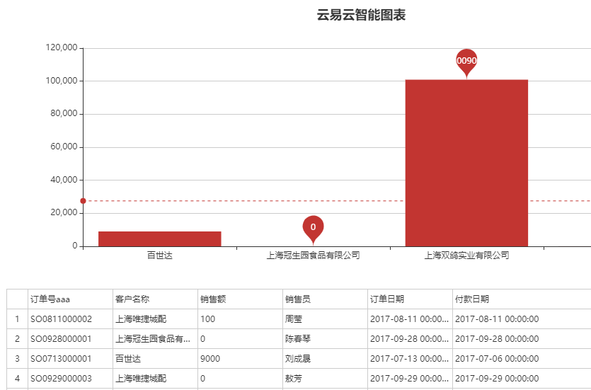
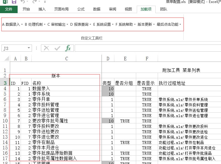
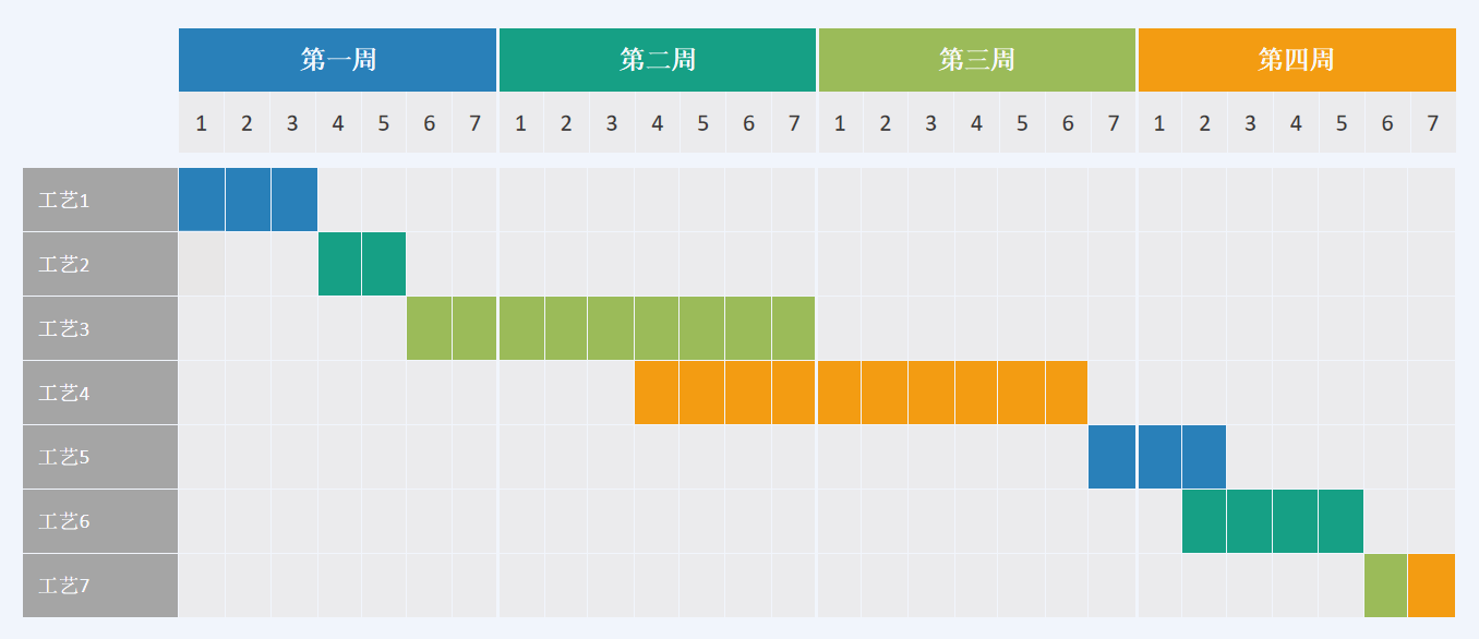
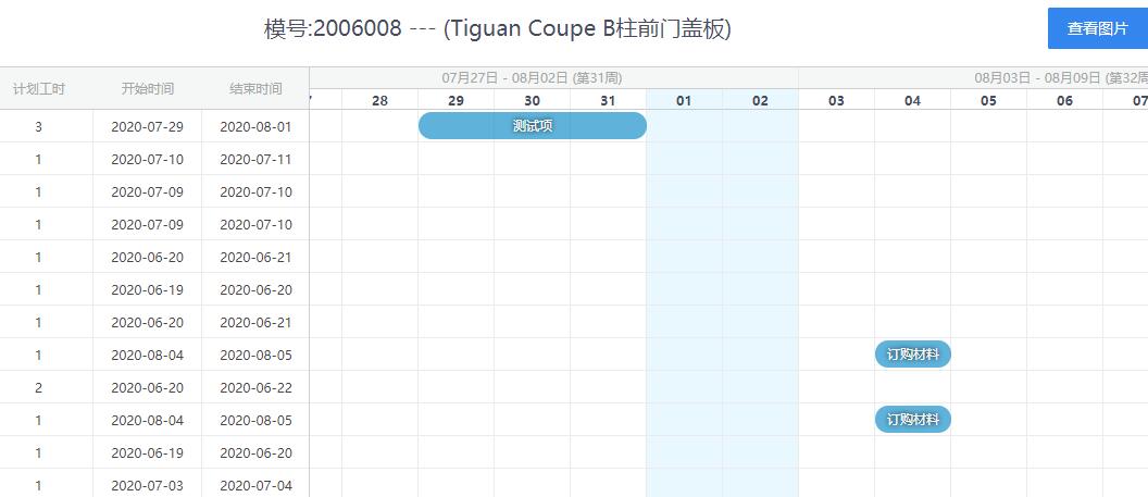
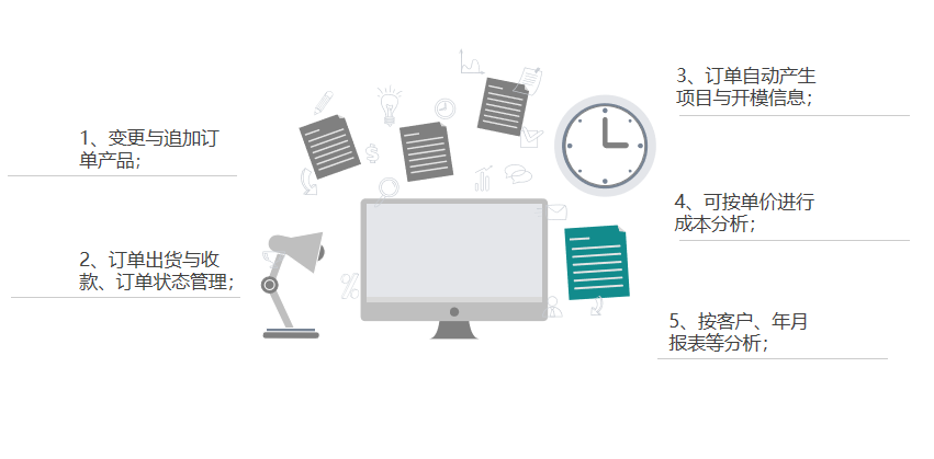
模具管理中有生产绩效报表，进度报表、产能负荷报表、机台负荷报表等等，将数据进行分组汇总后，看到的数据还是不够直观，所以要进行图表的建立。如果要生成每个模号的图表。

第一种方式：建立模板文件，将数据复制进去即可形成图表，这里的前提是分组的数据要用公式先设置好，如果分组是动态的，或者不显示零值的数据。那么就要采用第二种方式。

第二种方式：通过取数据库数据，然后在excel菜单中点击按钮进行拉取数据，过滤处理后，然后进行分组统计，最后显示数据和图表，这样数据是最新格式，可按程序指令进行格式处理，保证数据的准确安全。并且运行速度是最快的。

云易云软件基于数据库管理系统，Excel相结合的方式进行模具管理与生产绩效报表分析。Excel的便捷在于，报表的深度加工处理，很多管理系统都无法调整到个性化级别。以及报表电子档方式发送到客户供应商。对于上游客户需要进行产量、质量报备的情况下。数据库与VBA代码可提供管理信息系统的改造，实现企业的生态化管理。

以下为生成图表的源码，有问题可咨询QQ：53757591 Private Sub 生成图表(ByVal sh As String, ByVal a1 As Integer, ByVal a2 As Integer, ByVal tol As Long) Dim mychart As String Dim i As Integer ActiveWindow.ScrollRow = 1 ActiveWindow.ScrollColumn = 1     Charts.Add     mychart = ActiveChart.Name     ActiveChart.ApplyCustomType ChartType:=xlBuiltIn, TypeName:="两轴线-柱图"     ActiveChart.SetSourceData Source:=Sheets(sh).Range("A65536"), PlotBy _         :=xlColumns     ActiveChart.SeriesCollection.NewSeries     ActiveChart.SeriesCollection.NewSeries     ActiveChart.SeriesCollection(1).XValues = "='" & sh & "'!R" & a1 & "C2:R" & a2 & "C2"     ActiveChart.SeriesCollection(1).Values = "='" & sh & "'!R" & a1 & "C3:R" & a2 & "C3"     ActiveChart.SeriesCollection(2).Values = "='" & sh & "'!R" & a1 & "C9:R" & a2 & "C9"     ActiveChart.Location where:=xlLocationAsObject, Name:=sh     ActiveChart.ApplyCustomType ChartType:=xlBuiltIn, TypeName:="两轴线-柱图"     With ActiveChart         .HasTitle = False         .Axes(xlCategory, xlPrimary).HasTitle = True         .Axes(xlCategory, xlPrimary).AxisTitle.Characters.Text = "不良项目"         .Axes(xlValue, xlPrimary).HasTitle = True         .Axes(xlValue, xlPrimary).AxisTitle.Characters.Text = "不良数"         .Axes(xlCategory, xlSecondary).HasTitle = False         .Axes(xlValue, xlSecondary).HasTitle = True         .Axes(xlValue, xlSecondary).AxisTitle.Characters.Text = "累积影响度"     End With     ActiveChart.HasLegend = False     ActiveChart.Axes(xlValue).AxisTitle.Select     With Selection         .HorizontalAlignment = xlCenter         .VerticalAlignment = xlCenter         .ReadingOrder = xlContext         .Orientation = xlVertical     End With     ActiveChart.Axes(xlValue, xlSecondary).AxisTitle.Select     With Selection         .HorizontalAlignment = xlCenter         .VerticalAlignment = xlCenter         .ReadingOrder = xlContext         .Orientation = xlVertical     End With     ActiveChart.Axes(xlValue).Select     With ActiveChart.Axes(xlValue)         .MinimumScale = 0         .MaximumScale = tol         .MinorUnit = 4         .MajorUnit = tol / 5         .Crosses = xlAutomatic         .ReversePlotOrder = False         .ScaleType = xlLinear         .DisplayUnit = xlNone     End With     ActiveChart.Axes(xlValue, xlSecondary).Select     With ActiveChart.Axes(xlValue, xlSecondary)         .MinimumScale = 0         .MaximumScale = 100         .MinorUnit = 25         .MajorUnit = 25         .Crosses = xlAutomatic         .ReversePlotOrder = False         .ScaleType = xlLinear         .DisplayUnit = xlNone     End With     ActiveChart.SeriesCollection(1).Select     With Selection.Border         .Weight = xlThin         .LineStyle = xlAutomatic     End With     Selection.Shadow = False     Selection.InvertIfNegative = False     Selection.Interior.ColorIndex = xlNone     With ActiveChart.ChartGroups(1)         .Overlap = 0         .GapWidth = 0         .HasSeriesLines = False         .VaryByCategories = False     End With     ActiveChart.PlotArea.Select     With Selection.Border         .ColorIndex = 16         .Weight = xlThin         .LineStyle = xlContinuous     End With     Selection.Interior.ColorIndex = xlNone     For i = 1 To ActiveSheet.ChartObjects.Count         ActiveSheet.ChartObjects(i).Select         ActiveChart.ChartArea.Select         ActiveSheet.Shapes(i).Left = Range("J31").Left         ActiveSheet.Shapes(i).Top = Range("J31").Top         ActiveSheet.Shapes(i).Width = Range("S43").Left - Range("J31").Left         ActiveSheet.Shapes(i).Height = Range("S43").Top - Range("J31").Top     Next i End Sub